We want to create a planet-size digital place with dynamic time of day. Atmospheric scattering is an indispensable effect for rendering a realistic planet. It's the most important part of the sky, one of our primary light sources.
"The sky color gives key indications about the hour of the day, and the aerial perspective gives an important cue to evaluate distances." - [3]
Author: Ruby (DongJi) Render Programmer

How do we implement it?
We do it iteratively.
Iteration 1 - Reconstruct the position from the depth buffer
We do it in a compute shader. To sample from the depth buffer, we also need to create an SRV (Shader Resource View) with R32_FLOAT format from the depth buffer.
First, we can use UV and depth to get the position in clip space. Then we use the inverse (local) view projection matrix to get the position in world space.
See Figure 1, code is provided in Appendix A.


Figure 1: Output local world space position
To test the result, we use the reconstructed position to generate the fog.

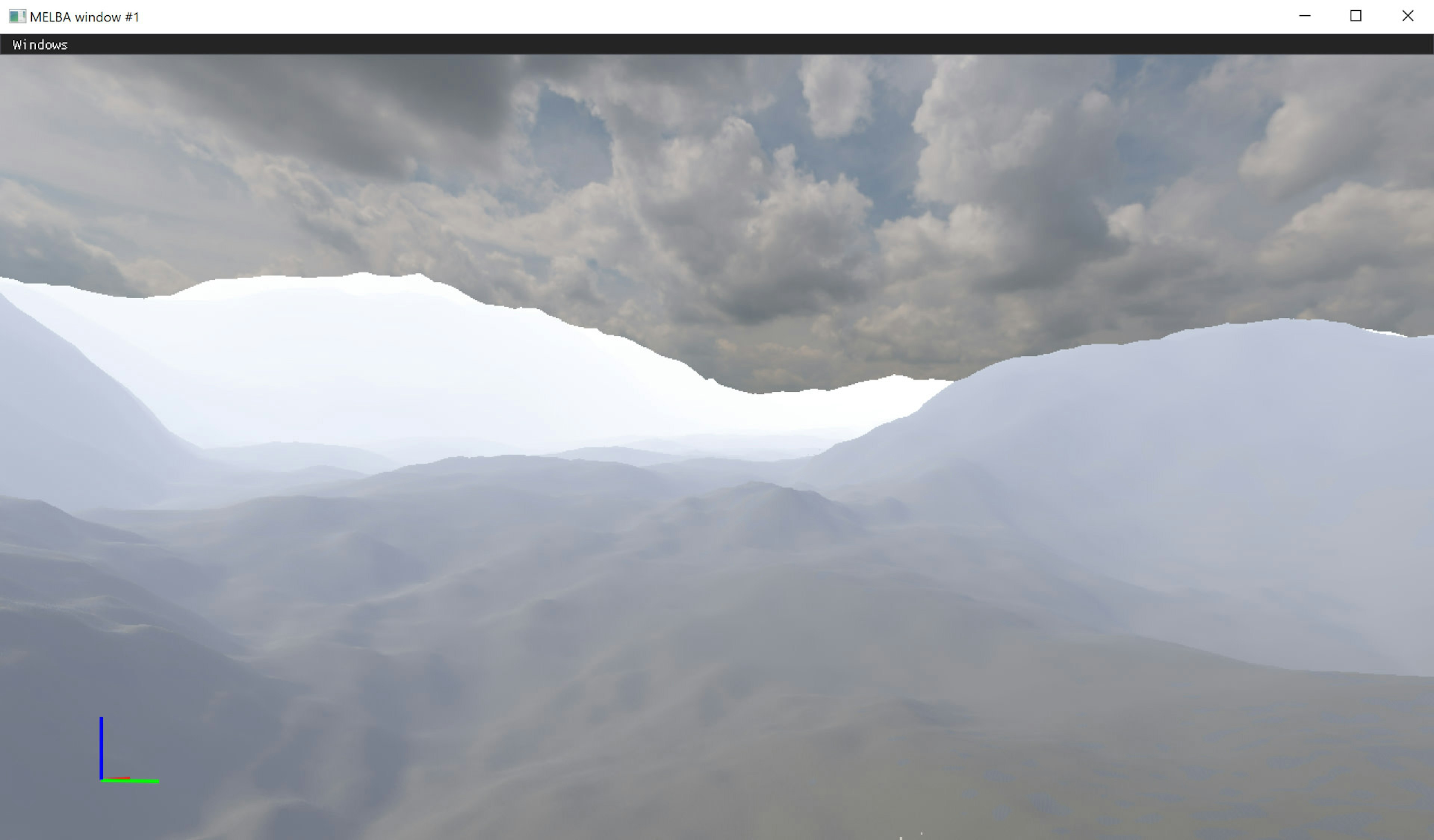
Figure 2: Test with fog
Iteration 2 - Implement Nishita93 model with brute force ray marching
We decided to start with the Nishita93 model [1]. It's a single scattering model.
We do ray marching in two directions: view direction and light direction. For view direction, if some part of it does not get the light from the sun, other parts can still receive and transfer the energies. For light direction, if we notice that any part of the ray is occluded, we can immediately stop the calculation and throw away the accumulated results since the light from the sun won't be able to do any contribution in this case. So we should go through it thoroughly.
Parameters
Planet radius: We use 6371 km.
Planet center: We use (0, 0, 0) since we only have one planet for now. We can use different values in the future.
Atmosphere height: We use 80 km as the height/thickness of the atmosphere, where the mesosphere locates.
Density scale height (Rayleigh): We use 7994 m.
Density scale height (Mie): We use 1200 m.
Scattering coefficient (Rayleigh): We calculate to get this parameter on the C++ side. First, we use the index of refraction of the atmosphere (at sea level) n = 1.0003 on the C++ side. First, we use the index of refraction of the atmosphere (at sea level) and the Rayleigh particles' molecular number density of the atmosphere (at sea level) Ns = 2.55e25 to calculate the Rayleigh constant. Then we use this Rayleigh constant and wavelength = (680, 550, 440) nm [4] to calculate the scattering coefficient. Code is provided in Appendix B.


Scattering coefficient (Mie): We use (0.00002, 0.00002, 0.00002) [3].
Implementation
We launch the 1st ray, starting from the camera position along the view direction. Then we get the intersection points between this ray and the outer atmosphere. Now we will get the path we want ray marching on.

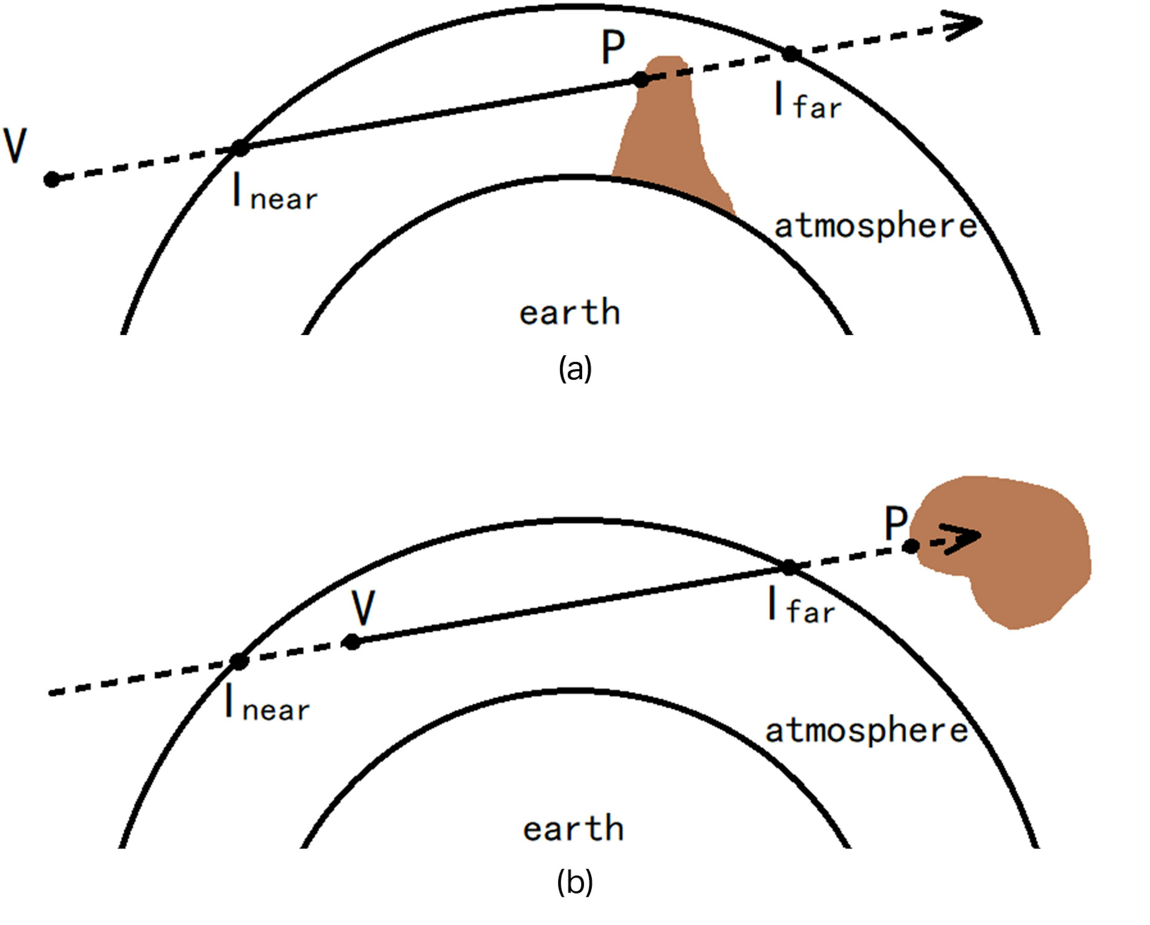
Figure 3: Get the path on 1st ray
See Figure 3. V is the camera position. P is the fragment position which we reconstructed in the 1st iteration. Inear and Ifar are the intersections. If V is outside the atmosphere, we will pick Inear as the path's starting point. If V is inside the atmosphere, we will pick it as the path's starting point. In either case, we choose the more progressed point (either V or Inear) on the ray as the start point. Similarly, between P and Ifar, we pick the less progressed one on the ray as the path's endpoint.
Be aware that the path could be an invalid one. For example, see Figure 4; in this case, Inear should be the start point, and P should be the endpoint, which makes the path an invalid one along the ray direction. If the path on the 1st ray is invalid, just exit the calculation since there's no scattering contribution.
Code is provided in Appendix D.

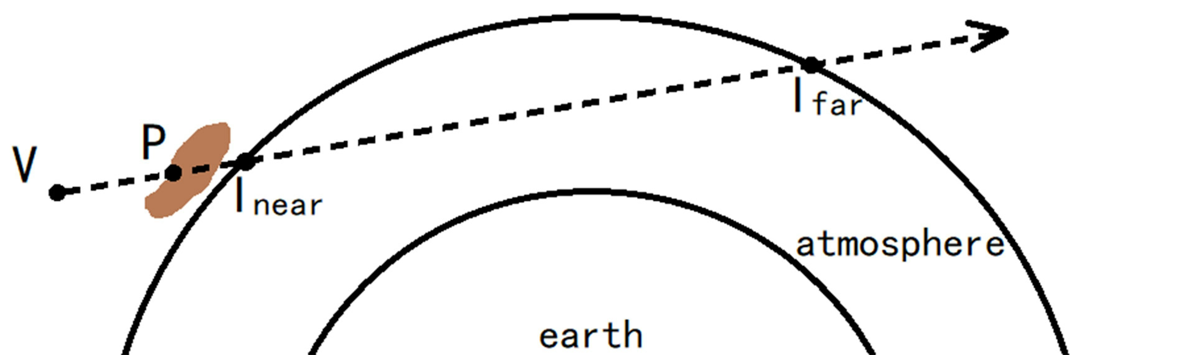
Figure 4: An invalid path
Now that we have the 1st ray, we can start to do the marching and integrate our in-scattering. For each step, we first get the density ratio at that point.

Then, starting from the point, we also calculate the optical depth along the sunlight direction. To get the optical depth along the sunlight direction, we launch the 2nd ray, which starts from the point and along the sunlight direction. If the planet blocks this ray, then there will be no contribution from this ray, see Figure 5 (a). Otherwise, we just need to clamp this ray inside the outer atmosphere, see Figure 5 (b). After the 2nd ray is prepared, we do ray marching and integrate the density ratio to get the optical depth. Code is provided in Appendix E.
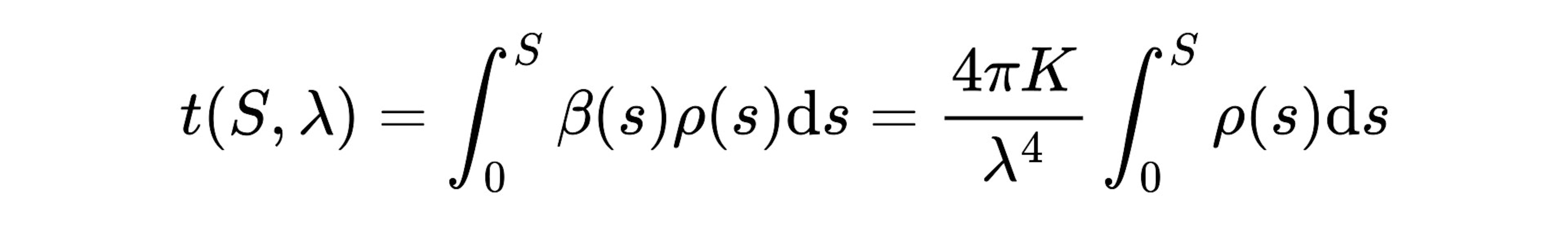

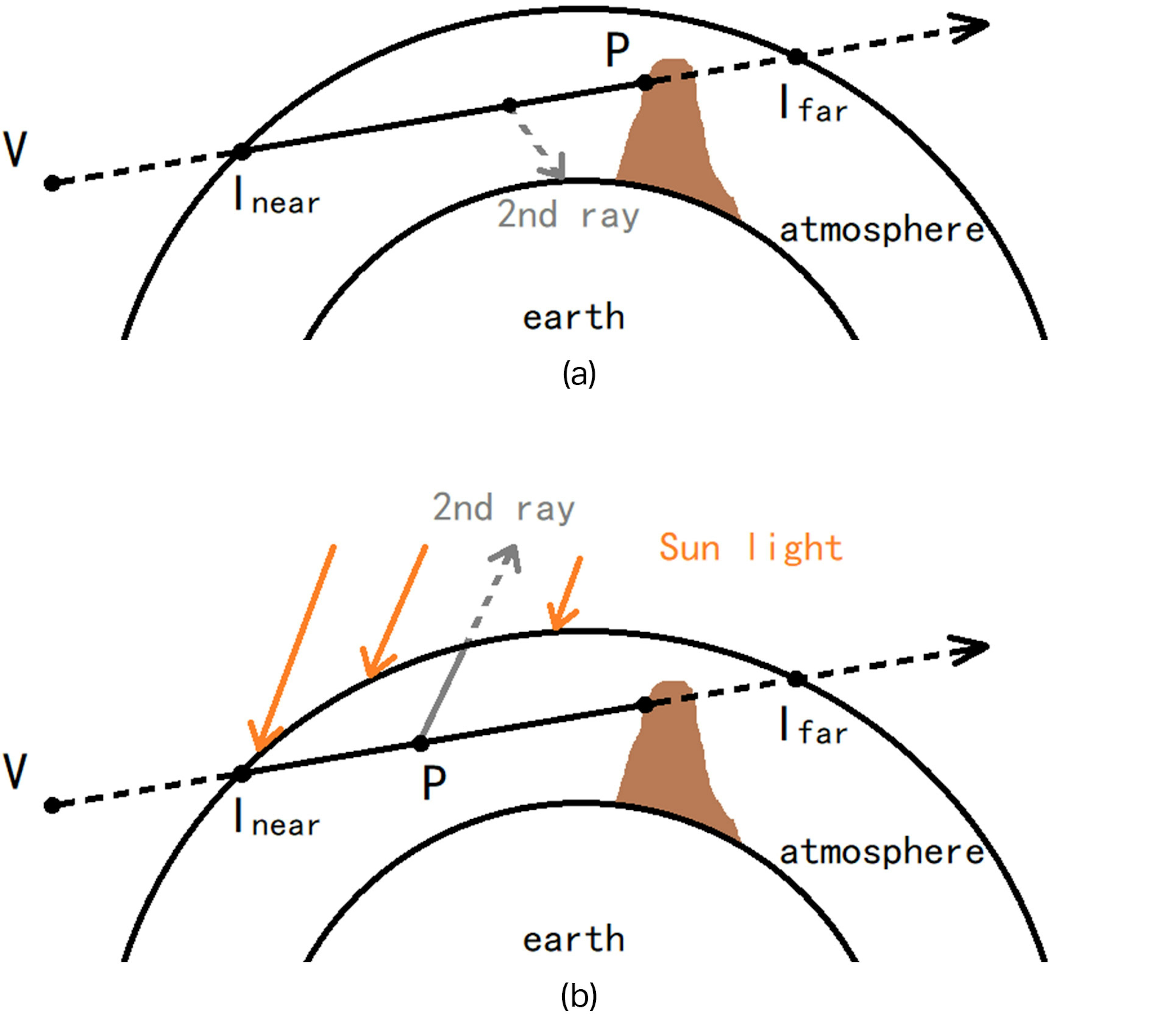
Figure 5: 2nd ray
We then use the density ratio and optical depth to compute the in-scattering at this point and integrate it. After the integration, we apply different corresponding phase functions to the Rayleigh in-scattering and Mie in-scattering parts. Code is provided in Appendix F.

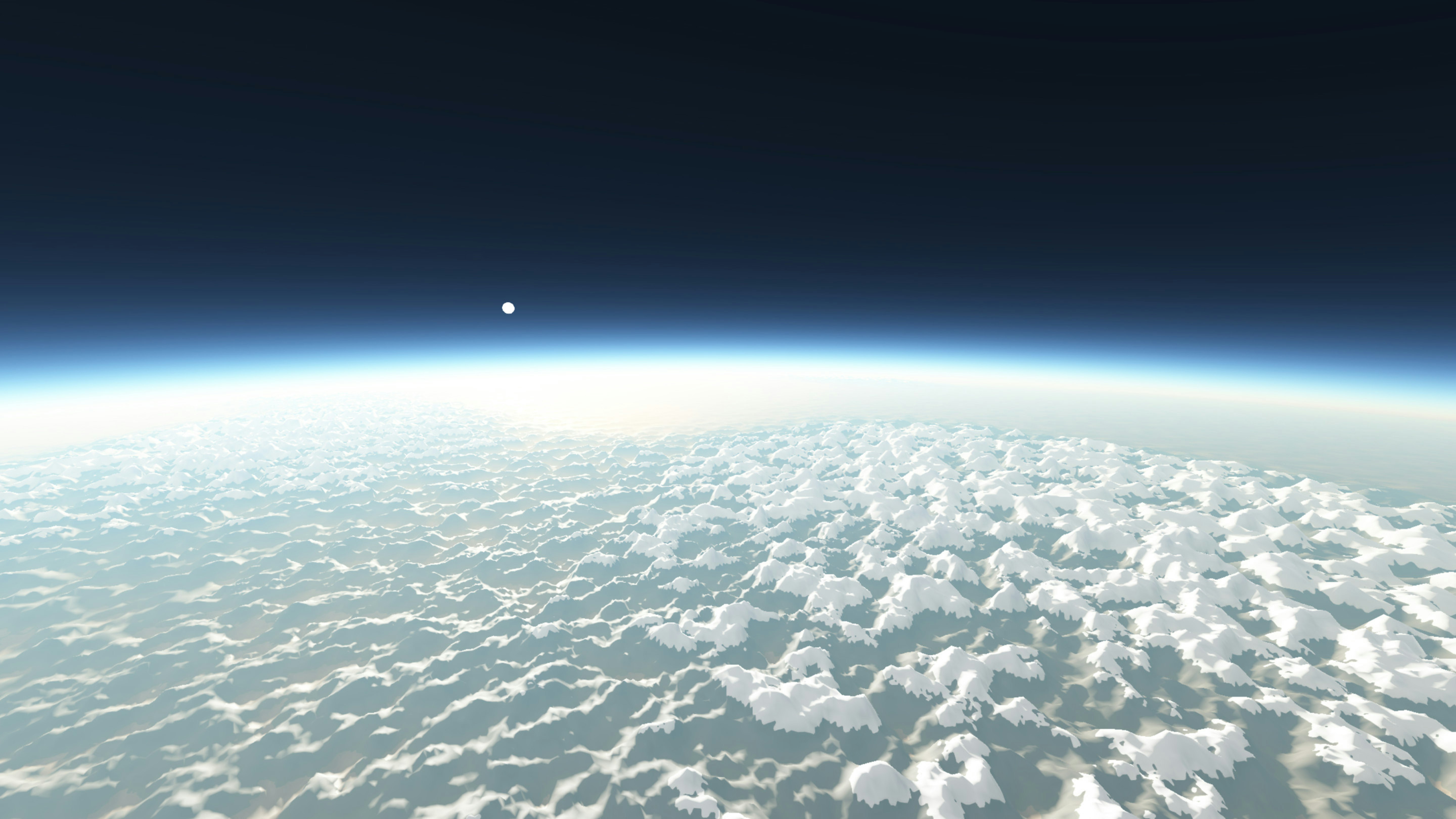
Finally, we calculate and combine the in-scattering, out-scattering and the lighting data in the light buffer to get our final scattering result. See Figure 6; now, the planet is starting to look good. Code is provided in Appendix G.

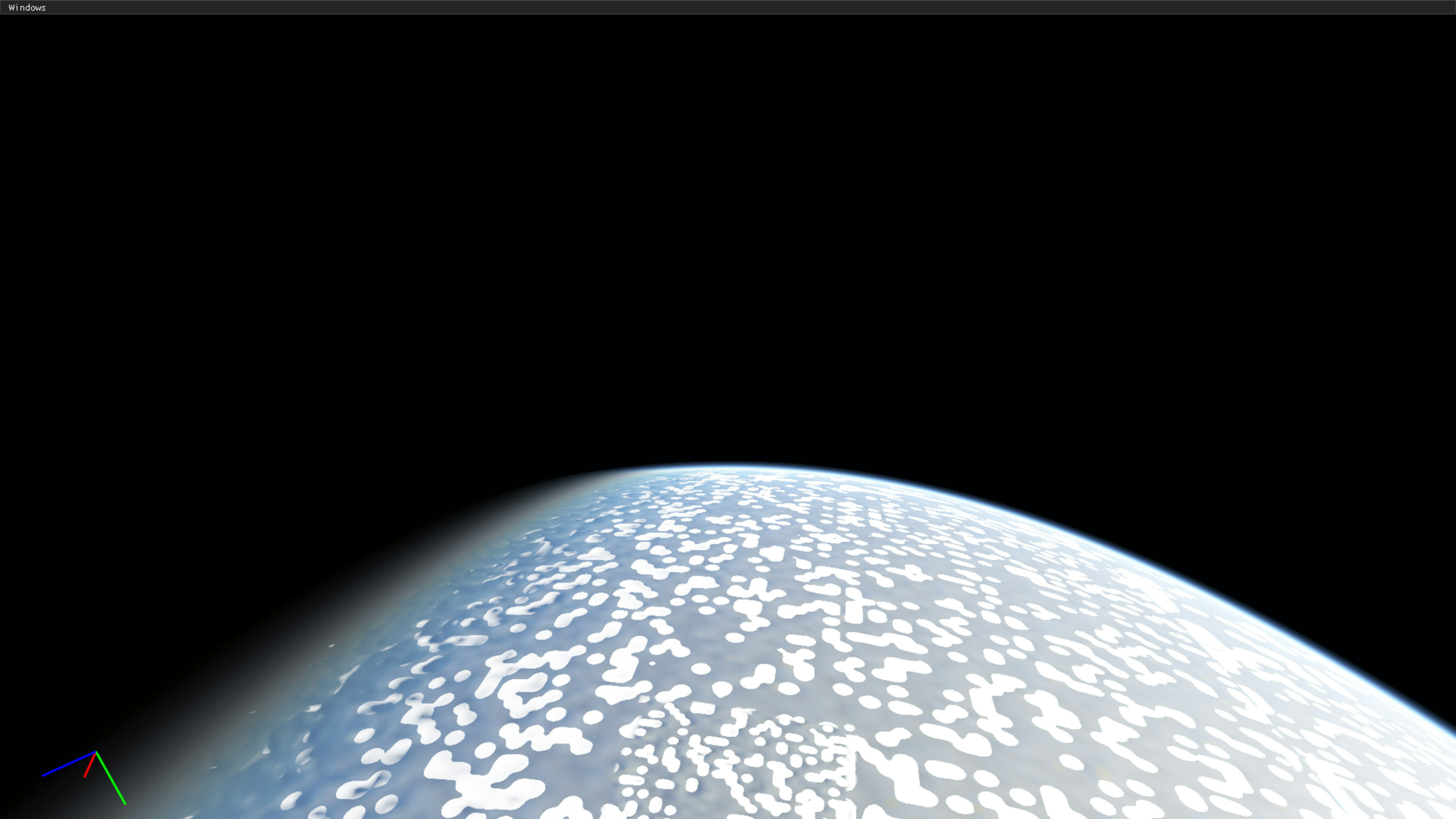
Figure 6: Now, the planet is starting to look good :D
Iteration 3 - Precomputation & minor improvements
First, we start by implementing the process of precomputation.
We decided to start with the 2D lookup table proposed by O'Neil in 2004, referenced below [2]. The lookup table is generated in another compute shader. We map UV.x from [0, 1] to [altitude on the ground, altitude at the top of the atmosphere] and map UV.y from [0, 1] to [cos(PI), cos(0)] (zenith angle). In the end, we store the related density ratio and the optical depth (along the direction) in the lookup table. Code is provided in Appendix H.
Performance is around 10 times faster with precomputation. See one of the previous test cases in Figure 7. In this case, the original version costs 6.64 ms, while the new pre-computation version only costs 0.69 ms.

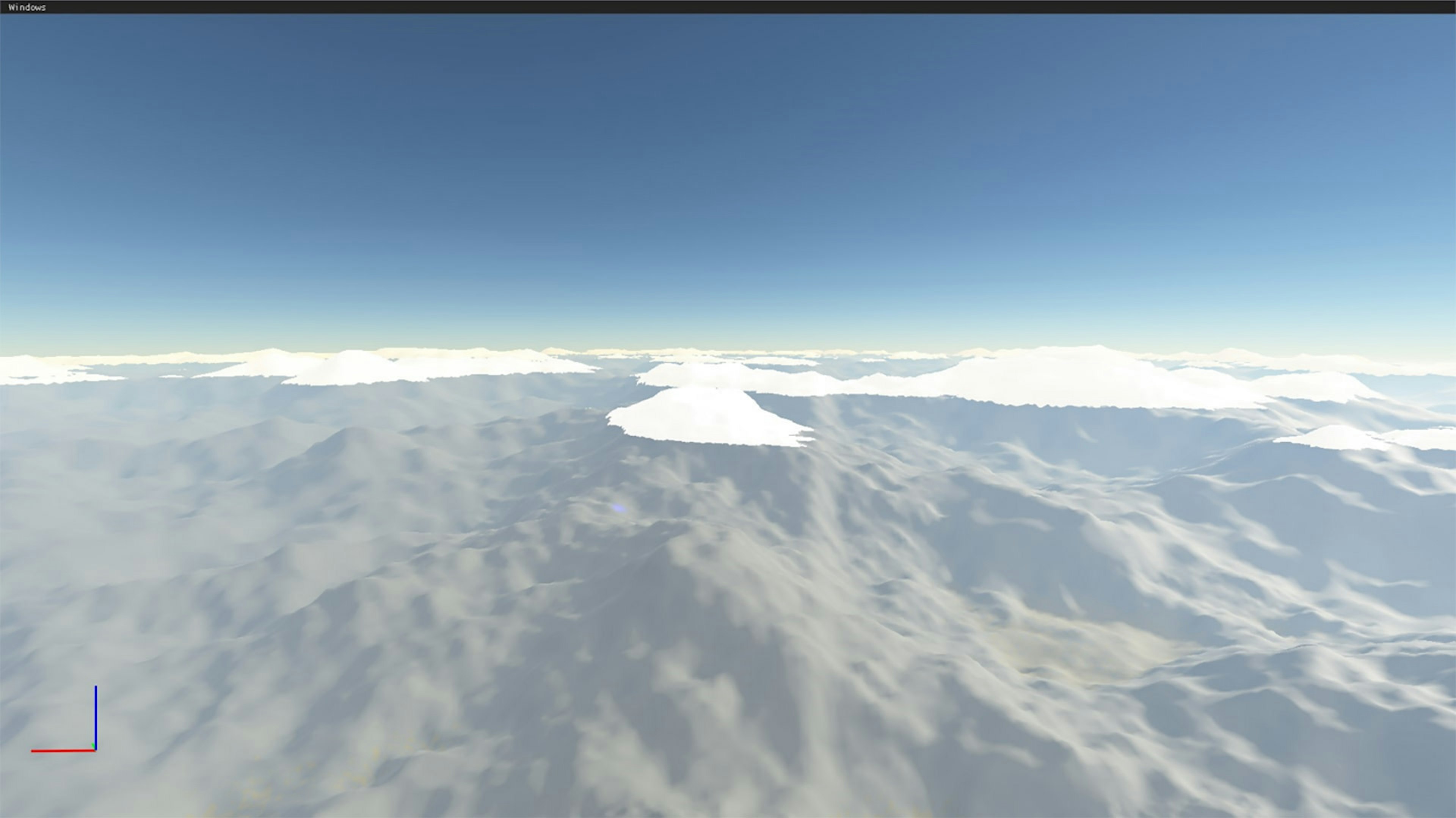
Figure 7: The view when testing performance
Then we add the sun disk. Having a sun disk is important as it is how it looks in the real world. See the lovely view of the sun disk in Figure 8. A fun fact is that the angular size of the Sun and the Moon are pretty close (~ 0.5o = 30 arcmin) if viewed from the Earth's surface [4].
Figure 8: Nice views of the sundisk
Finally, we use a configurable extra-terrestrial solar irradiance with 3 constants [5]. We multiply 3 spectrum samples L(λr), L(λg), and L(λb) by these 3 constants to get the RGB color. This gives us a relatively accurate approximation compared to spectral rendering with a large number of wavelengths [6]. See the difference between before and after in Figure 9.
In computer graphics, spectral rendering is a technique in which a scene's light transport is modelled with actual wavelengths [7].


Figure 9a: Before & after spectral rendering


Figure 9b: Before & after spectral rendering
Future improvements
The next iteration aims to add multiple scattering, and some parameter values (such as the thickness of the atmosphere) may be adjusted. We also plan to extend the method to support non-opaque objects (transparent, volumetric, etc.).
For the challenges/features we see in the future, we need to think about how to integrate the weather with atmospheric scattering on our planet. I assume this step will be challenging.
If you are interested in joining us to tackle these challenges or even invent an entirely novel solution, then check out our career page.
Reference
[1] Nishita 1993, Display of The Earth Taking into Account Atmospheric Scattering -
http://nishitalab.org/user/nis/cdrom/sig93_nis.pdf
[2] O’Neil, Accurate Atmospheric Scattering - https://developer.nvidia.com/gpugems/gpugems2/part-ii-shading-lighting-and-shadows/chapter-16-accurate-atmospheric-scattering
[3] Bruneton & Neyret 2008, Precomputed Atmospheric Scattering - https://hal.inria.fr/inria-00288758/document
[4] Angular Diameter - https://www.astronomy.swin.edu.au/cosmos/A/Angular+Diameter
[5] Precomputed Atmospheric Scattering: a New Implementation - https://ebruneton.github.io/precomputed_atmospheric_scattering/
[6] A Qualitative and Quantitative Evaluation of 8 Clear Sky Models - https://arxiv.org/pdf/1612.04336.pdf
[7] Spectral rendering - Spectral rendering
Appendix A
Reconstruct position from UV and depth
Appendix B
Calculate the Rayleigh constant
Appendix C
Ray sphere intersection
Appendix D
Get the path to ray march on the 1st ray
Appendix E
Get optical depth along the light direction
Appendix F
Phase function
Appendix G
Combine everything and get the final scattering result
Appendix H
Generate lookup table